Supply, Demand, and Government Intervention
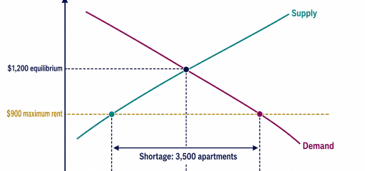
The Chapter 5 companion lesson study guide on Effortless Math covers Supply, Demand, and Government Intervention: the key terms, the core ideas, and worked examples showing how this topic is tested on this course.
Chapter 5 companion lesson
A rent ceiling, a tax on sellers, and a surge in buyer income can all change a market, but not in the same way. The first job is to identify the curve or constraint that actually changes.
In plain language: Supply and demand determine a competitive market's equilibrium price and quantity. A change in the good's own price creates movement along a curve; a change in another determinant shifts the curve. Price controls, taxes, subsidies, and tariffs alter incentives and can create shortages, surpluses, tax wedges, or deadweight loss.
Why does demand, quantity demanded, and demand shifters matter?
Demand is a schedule showing how much buyers are willing and able to purchase at different prices during a stated period, other things equal. Quantity demanded is one amount at one price. The distinction separates a whole relationship from a point on it. When a good's own price changes, buyers move along the demand curve. When another determinant changes, the entire curve shifts.
Demand usually slopes downward. At a lower price, existing buyers may purchase more, additional buyers may enter, and consumers may substitute toward the good and away from alternatives. The income effect of a price change can also raise purchasing power. Introductory analysis groups these mechanisms into the law of demand without requiring the curve to be straight.
Income shifts demand differently for normal and inferior goods. Higher income raises demand for a normal good and lowers demand for an inferior good. “Inferior'' is a technical classification, not a statement about quality. Bus rides might be inferior for commuters who buy cars when income rises, while remaining normal for other consumers or settings. The stem must provide or imply the classification.
How does the CLEP test supply, quantity supplied, and supply shifters?
Supply is a schedule showing how much sellers are willing and able to offer at different prices during a stated period, other things equal. Quantity supplied is one amount at one price. A higher own price usually raises quantity supplied along the curve because producing additional units becomes worthwhile. A change in production conditions shifts the entire supply relationship.
Input prices are central shifters. If wages, energy, raw materials, or financing costs rise, producing each quantity becomes more costly and supply shifts left. Lower input costs shift supply right. A change in a worker's wage is an input-cost event for the product market, not a movement caused by the product's own price.
Technology raises the amount that can be produced from given inputs or reduces unit cost, shifting supply right. The improvement must be relevant to the production process. Better wheat seeds shift wheat supply; they do not automatically shift demand for wheat. Productivity improvements later reappear as rightward SRAS or LRAS shifts at the macro level.
Watch the model in motion
Jacob Clifford explains the same core relationship visually. Pause before each result and predict the next movement or calculation.
What should you know about equilibrium, shortage, surplus, and simultaneous shifts?
Market equilibrium occurs where quantity demanded equals quantity supplied. Buyers' planned purchases match sellers' planned sales at the equilibrium price. The price coordinates plans; it does not guarantee equal income, moral fairness, or absence of external costs. Efficiency claims require assumptions about competition, information, and spillovers.
At a price below equilibrium, quantity demanded exceeds quantity supplied, creating a shortage. Buyers compete for limited units, wait, search, or offer more, placing upward pressure on price when adjustment is allowed. At a price above equilibrium, quantity supplied exceeds quantity demanded, creating a surplus. Unsold goods encourage sellers to cut price or reduce production.
Calculate the amount of shortage or surplus by subtraction at the controlled or stated price. If 900 units are demanded and 620 supplied, the shortage is 280, not 620 or 1,520. The transaction quantity cannot exceed the short side of the market; in this example, at most 620 units trade without another allocation mechanism.
How does the CLEP test binding price ceilings and price floors?
A price ceiling is a legal maximum. It is binding only when set below the equilibrium price. A ceiling above equilibrium does not constrain the market because the equilibrium price already satisfies the law. A binding ceiling holds price below the level that would equate quantity demanded and supplied, creating a shortage.
A price floor is a legal minimum. It is binding only when set above equilibrium. A floor below equilibrium is nonbinding. A binding floor leaves quantity supplied greater than quantity demanded, creating a surplus. The minimum wage is a price floor in a labor-market model: the price is the wage, firms demand labor, and households supply it. Under the simple competitive model, a binding minimum wage creates excess labor supplied, or unemployment in that market.
The welfare effects depend on which transactions occur and how rationing works. Under a binding ceiling, some buyers who value the good highly may be unable to obtain it, and sellers provide fewer units. Search and queuing costs can absorb part of the apparent price reduction. Quality may fall if sellers cannot charge for improvements. A black market may arise. These are possible responses, not logical requirements in every setting.
How does the CLEP test taxes, subsidies, elasticity, and tariffs?
A per-unit tax creates a wedge between the price buyers pay and the amount sellers receive. The quantity traded falls because the wedge discourages both purchase and production. Drawn as a shift of supply, the after-tax supply curve lies above the original by the tax per unit. At the new quantity, the vertical distance between buyer and seller prices equals the tax.
Tax incidence describes who bears the economic burden, not who sends the payment to the government. The less responsive side bears more because it cannot avoid the taxed activity easily. If demand is relatively inelastic, buyers continue purchasing despite a higher price and bear more. If supply is relatively inelastic, sellers cannot shift resources readily and absorb more through a lower net price.
Elasticity measures responsiveness. Perfectly inelastic demand is vertical: quantity does not respond to price, so buyers bear a per-unit tax in the extreme model. Perfectly elastic demand is horizontal: buyers will not pay above the market price, so sellers bear it. Most markets lie between these cases. A steeper line is not always less elastic because elasticity also depends on scale and the point measured; exam graphs usually provide enough context for a qualitative comparison.
What is the CLEP likely to ask?
Expect curve shifts, movement-versus-shift language, binding controls, shortage or surplus calculations, tax incidence, and tariff effects. For two simultaneous shifts, state the separate effect of each on price and quantity before choosing what is certain.
A useful check is to name the model before doing arithmetic. Then write the first change, the intermediate market response, and the final macroeconomic result. This keeps a plausible distractor from borrowing one true step and attaching it to the wrong conclusion.
Can you do these without notes?
- For each event, say whether demand shifts and in which direction: income rises for a normal good; the good's own price falls; a complement's price rises; buyers expect a future shortage; and the number of buyers falls.
- Distinguish a fall in supply from a fall in quantity supplied. Then predict the supply shift from lower energy costs, a producer tax, improved technology, expected higher future price for a storable good, and entry of new sellers.
- For each pair, state the certain result and the indeterminate result: demand rises with supply falling; demand and supply rise; demand falls with supply rising; and demand and supply fall.
For each prompt, say why the tempting wrong answer fails. That extra sentence is often the difference between recognizing a term and being able to use it under time pressure.
Keep studying with the complete guide
This lesson accompanies CLEP Principles of Macroeconomics for Beginners. The book adds annotated graphs, worked calculations, chapter practice, two printed full-length tests, and ten online test forms.

Reza is an experienced Math instructor and a test-prep expert who has been tutoring students since 2008. He has helped many students raise their standardized test scores--and attend the colleges of their dreams. He works with students individually and in group settings, he tutors both live and online Math courses and the Math portion of standardized tests. He provides an individualized custom learning plan and the personalized attention that makes a difference in how students view math.
Related to This Article
More math articles
- How to Use the Pythagorean Theorem (Real-World Examples)
- Proportions Practice — Solve for the Unknown (Free)
- Conformity, Obedience, and Situational Influence
- How is the SSAT Test Scored?
- Best Calculators for Algebra
- 10 Most Common 6th Grade MCAS Math Questions
- Geometry Puzzle – Challenge 70
- FREE 6th Grade Georgia Milestones Assessment System Math Practice Test
- Teenager’s Books That Make Math Fun
- Top 10 Tips to Create a TABE Math Study Plan



















What people say about "Supply, Demand, and Government Intervention"?
No one replied yet.