Hardy-Weinberg Calculations: Equations and Worked Examples
Hardy-Weinberg calculations use allele frequencies \(p+q=1\) and predicted genotype frequencies \(p^2+2pq+q^2=1\). First identify what the data count. A recessive phenotype frequency can be square-rooted to find \(q\) only under the stated model and equilibrium assumptions; complete genotype counts allow direct allele counting.
Here is a question you can answer with a coin. If a population’s gene pool is 70 percent \(A\) and 30 percent \(a\), and eggs and sperm meet at random, what fraction of the offspring should be heterozygous? You are drawing two alleles at random, so this is the same problem as flipping a weighted coin twice. The probability calculation follows from random pairing. Hardy-Weinberg analysis also asks whether the conditions supporting stable frequencies hold.
Watch the process
Solving Hardy-Weinberg Problems
The Hardy-Weinberg model supplies a baseline for comparing allele and genotype frequencies. It predicts stable allele frequencies under specified conditions and gives the genotype proportions expected from random union of gametes. A departure tells you that the population differs from the model. It does not, by itself, identify the cause.
The Two Expressions
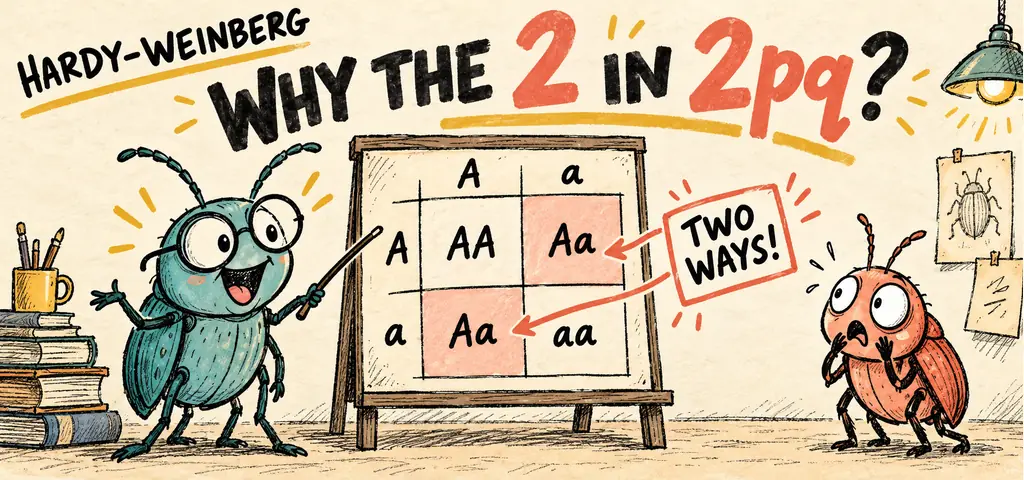
Consider one gene with two alleles. Let \(p\) be the frequency of one and \(q\) the frequency of the other. Because every allele at that locus is one or the other, \[p + q = 1 .\] Now build genotypes. Random mating in a large population is equivalent to throwing all the gametes into one bucket and drawing two at a time, because a sperm has no way of knowing which egg it will meet. For this standard autosomal model, assume the frequency of \(A\) is the same, \(p\), among sperm and eggs. Lay the two out as a gamete table, which is a Punnett square whose entries are frequencies rather than counts:
| egg \(A\) (freq. \(p\)) | egg \(a\) (freq. \(q\)) | |
|---|---|---|
| sperm \(A\) (freq. \(p\)) | \(AA\): \(p \times p = p^2\) | \(Aa\): \(p \times q = pq\) |
| sperm \(a\) (freq. \(q\)) | \(Aa\): \(q \times p = pq\) | \(aa\): \(q \times q = q^2\) |
Read the four cells. Two independent draws of \(A\) give \(AA\) at frequency \(p^2\). Two independent draws of \(a\) give \(aa\) at frequency \(q^2\). The heterozygote appears in two cells, once from an \(A\) sperm meeting an \(a\) egg and once from an \(a\) sperm meeting an \(A\) egg, so its total frequency is \(pq + pq = 2pq\). The factor of 2 counts the two routes to the heterozygous genotype. Include both routes in the probability.
The four cells are every possible outcome, so they must sum to one: \[p^2 + 2pq + q^2 = 1 .\] You can also get there algebraically, which is worth seeing once. Since \(p + q = 1\), squaring both sides gives \((p+q)^2 = 1^2\), and expanding the left side gives \(p^2 + 2pq + q^2 = 1\). This algebraic identity holds whenever \(p+q=1\). Interpreting its terms as actual genotype frequencies requires the random-union assumptions; algebra alone does not show that a population fits the model. The second expression is the first one squared, which is why the two are always used together and why a value of \(p\) you have not checked against \(p + q = 1\) is a value you should not trust. The AP reference sheet supplies these expressions and symbol definitions. Label what each represents in your own calculation: \(p\) and \(q\) are allele frequencies, while \(p^2\), \(2pq\), and \(q^2\) are genotype frequencies. Label each quantity before substituting a number.
The Five Conditions
The standard idealized model predicts stable allele frequencies and Hardy-Weinberg genotype proportions under the following sufficient conditions. A matching pattern alone does not prove all five hold; opposing processes can balance. Each is the absence of a mechanism that would change the population, which is the useful way to remember them.
-
No mutation. No alleles are created or converted into others.
-
No gene flow. No alleles are exchanged with other populations through successful reproduction.
-
No natural selection. All genotypes reproduce equally well.
-
Random mating. Mates pair without regard to genotype at the locus.
-
Very large population size. Large enough that drift is negligible.
To apply the model, take each condition and say exactly what it forbids and what a violation would look like in data.
No mutation forbids any change in the identity of an allele: if \(A\) mutates to \(a\), \(p\) falls slightly each generation. Typical per-locus mutation rates are low, so evaluate whether mutation alone could account for the size of the observed change.
No gene flow forbids alleles crossing the population boundary in either direction. The signature is a frequency moving toward that of a neighboring population, provided migrants reproduce. Census size can stay constant if arrivals balance losses. An island is not automatically genetically isolated; look for an explicit absence of successful immigration.
No natural selection forbids any difference in survival or reproduction among genotypes. Evidence for a violation includes a loss or gain concentrated in one genotype class: the \(aa\) count falls while the others hold, or the heterozygotes out-reproduce both homozygotes. Note what the condition actually requires. It is not enough that all genotypes survive; they must leave equal numbers of offspring on average.
Random mating forbids mate choice that depends on the genotype at this locus. It does not forbid choosiness in general. A population where females choose males by territory quality is still mating at random with respect to a flower-color or blood-type locus, provided territory quality is unrelated to it. A heterozygote count departing from \(2pq\) can be consistent with nonrandom mating, but mating records or other evidence are needed to distinguish it from selection and population structure.
Very large population size forbids sampling error large enough to move frequencies. There is no threshold to memorize. The condition is really a statement that drift is negligible, so when a stem names a population of 30 and reports a swing of 0.2 in one generation, drift is on the table, and the same swing is much less likely if effective population size is 50,000. Census size alone does not establish effective size or eliminate chance.
No real population meets all five exactly, which is not a flaw. The model earns its keep as a baseline: when genotype frequencies fit the predictions you have no detected departure from those proportions at that locus, and when they do not, or when allele frequencies shift between generations, the deviation tells you where to look.
Choose the Quantity to Calculate
Begin by identifying the supplied quantity and the assumptions that connect it to an allele or genotype frequency.
First, establish the model: the phenotype shortcuts below assume an autosomal locus with two alleles, complete dominance, and a fully expressed recessive phenotype that identifies \(aa\). Then decide what the given number counts. A percentage of individuals showing the recessive phenotype is \(q^2\). A percentage of individuals showing the dominant phenotype is \(p^2 + 2pq\), which is \(1-q^2\). A percentage of alleles is \(p\) or \(q\) directly. Getting this step wrong makes every later step wrong, so label the number before you use it.
Second, choose the route supported by the data. Under Hardy-Weinberg equilibrium, take the square root of the recessive phenotype frequency to estimate \(q\). For a dominant phenotype frequency, subtract from one first. Without the equilibrium assumption, the observed recessive genotype frequency alone does not determine the allele frequency. If all genotype counts are known, count alleles directly: \(p=(2N_{AA}+N_{Aa})/(2N)\) and \(q=(2N_{aa}+N_{Aa})/(2N)\). This direct count does not require equilibrium.
Third, get \(p\) from \(p = 1-q\). Never square-root the dominant phenotype frequency to get \(p\); that shortcut is wrong because the dominant phenotype contains two genotypes.
Fourth, build what was asked. Heterozygote frequency is \(2pq\), homozygous dominant is \(p^2\), and a count is a frequency times population size. Check that the three genotype frequencies sum to one before answering.
Problem A, Allele Frequencies from a Recessive Phenotype
In a plant population of 1200, 108 plants show the recessive white flower phenotype and the rest are purple. Assuming Hardy-Weinberg equilibrium, calculate the dominant and recessive allele frequencies.
Start where the data let you start. Every white plant is homozygous recessive and no other genotype is white, so the observed frequency of white plants equals \(q^2\): \[q^2 = \frac{108}{1200} = 0.09, \qquad q = \sqrt{0.09} = 0.30, \qquad p = 1-q = 0.70 .\] The square root moves you from a genotype frequency to an allele frequency, and \(p + q = 1\) supplies the rest. Notice what you could not have done. Setting \(q = 0.09\) would confuse a genotype frequency with an allele frequency. Starting from the 1092 purple plants also works if you first calculate \(q^2=1-1092/1200=0.09\). What fails is taking the square root of the dominant phenotype frequency, because it combines two genotypes.
Answer
\(q = 0.30\) and \(p = 0.70\). For this recessive-phenotype problem, start with the observed homozygous recessive frequency and use the equilibrium assumption to identify it with \(q^2\). If allele frequencies or all genotype counts are supplied instead, use those data directly.
Problem B, Genotype Frequencies and Counting Carriers
A human population of 2500 is screened for a recessive metabolic disorder, and 100 people are affected. Assume a two-allele autosomal locus, complete penetrance, unaffected heterozygotes, and Hardy-Weinberg equilibrium. Predict each genotype frequency and the number of heterozygous carriers.
Get the allele frequencies first, by the same route as Problem A: \[q^2 = \frac{100}{2500} = 0.04, \qquad q = \sqrt{0.04} = 0.20, \qquad p = 1-0.20 = 0.80 .\] Now compute all three genotype frequencies: \[p^2 = (0.80)^2 = 0.64, \qquad 2pq = 2(0.80)(0.20) = 0.32, \qquad q^2 = (0.20)^2 = 0.04 .\] Check the sum first, because this is where an arithmetic slip shows itself: \(0.64 + 0.32 + 0.04 = 1.00\). Convert frequencies to counts by multiplying each by the population size: \[0.64 \times 2500 = 1600 \ \text{homozygous dominant}, \qquad 0.32 \times 2500 = 800 \ \text{carriers},\] \[0.04 \times 2500 = 100 \ \text{affected}, \qquad 1600 + 800 + 100 = 2500 .\] Eight hundred carriers hold the recessive allele while showing no sign of the disorder, against 100 affected individuals on whom selection can act. In this fully recessive model, selection against affected individuals has no direct fitness effect on copies carried by unaffected heterozygotes. This can slow the removal of a harmful recessive allele; actual persistence also depends on mutation, drift and other population processes.
Answer
\(p^2 = 0.64\) (1600), \(2pq = 0.32\) (800 carriers), \(q^2 = 0.04\) (100 affected). Most copies of a rare recessive allele sit in heterozygotes, where this fully recessive harmful effect does not lower heterozygote fitness.
Problem C, Testing Two Generations Against the Model
A biologist counts genotypes at one locus in two consecutive generations of a beetle population, each totaling 1000 individuals.
| AA | Aa | aa | |
|---|---|---|---|
| Generation 1 (observed) | 360 | 480 | 160 |
| Generation 2 (observed) | 490 | 420 | 90 |
Is this population at Hardy-Weinberg equilibrium across the two generations, and can these counts identify which mechanism caused the change?
Step 1: allele frequencies in Generation 1. There are 2000 alleles in the pool. Every AA individual contributes two \(A\) alleles and every Aa individual contributes one: \[p = \frac{2(360) + 480}{2000} = \frac{720 + 480}{2000} = \frac{1200}{2000} = 0.60, \qquad q = 1-0.60 = 0.40 .\]
Step 2: expected Generation 1 counts. Multiply each predicted frequency by 1000: \[p^2 = 0.36 \rightarrow 360, \qquad 2pq = 2(0.60)(0.40) = 0.48 \rightarrow 480, \qquad q^2 = 0.16 \rightarrow 160 .\] Observed and expected agree exactly, so Generation 1 alone gives no evidence of departure from the model.
Step 3: Generation 2. Repeat the count on the second row: \[p = \frac{2(490) + 420}{2000} = \frac{980 + 420}{2000} = \frac{1400}{2000} = 0.70, \qquad q = 1-0.70 = 0.30 .\]
Step 4: compare. The frequency \(p\) moved from 0.60 to 0.70 in one generation and \(q\) fell from 0.40 to 0.30. That is evolutionary change, so the population is not at Hardy-Weinberg equilibrium. Note the trap the data set is built around: testing Generation 2 against its own allele frequencies gives \(p^2 = 0.49 \rightarrow 490\), \(2pq = 0.42 \rightarrow 420\), and \(q^2 = 0.09 \rightarrow 90\), matching the observed counts perfectly. Matching genotype proportions within one generation does not establish stable allele frequencies across generations. Compare the allele-frequency measurements over time, accounting for sampling uncertainty.
Step 5: distinguish change from cause. The counts establish that \(p\) changed, but they do not uniquely identify selection, gene flow, drift, or mutation. Unchanged census size does not rule out gene flow: immigrants can replace emigrants or deaths. Census size also does not supply effective population size. Genotype-specific reproductive measurements and migration records would help identify the mechanism.
Interpreting the result
The population is not at equilibrium across generations: \(p\) rose from 0.60 to 0.70. Both rows nevertheless fit their own Hardy-Weinberg proportions. The mechanism cannot be identified from these counts alone.
Problem D, Entering Through the Dominant Phenotype
In a population of 800 beetles at Hardy-Weinberg equilibrium, 608 beetles show the dominant striped pattern and the rest are unstriped. How many beetles are expected to be heterozygous, and what fraction of all the striped beetles are heterozygous?
Follow the procedure. Step one, label the number. The 608 is a dominant phenotype count, which is \(p^2 + 2pq\) combined, so you cannot use it directly. Convert to the recessive class instead, because that class is a single genotype: \[800-608 = 192 \ \text{unstriped}, \qquad q^2 = \frac{192}{800} = 0.24 .\]
Step two, take the square root to move from a genotype frequency to an allele frequency: \[q = \sqrt{0.24} \approx 0.49 .\] This root is not exact, so check it rather than trusting the calculator blindly: \(0.49 \times 0.49 = 0.2401\), which is 0.24 to two decimal places. Round sensibly for display, but retain the calculator’s full precision for subsequent calculations and round the final result as requested.
Step three, get \(p\): \[p = 1-\sqrt{0.24} \approx 0.510102 .\]
Step four, build what was asked: \[2pq = 2(1-\sqrt{0.24})\sqrt{0.24} \approx 0.499796, \qquad 2pq \times 800 \approx 399.84 \approx 400 \ \text{heterozygotes}.\] As a rounded check: \(p^2 \approx 0.26\), \(2pq \approx 0.50\), \(q^2 = 0.24\), and \(0.26 + 0.50 + 0.24 = 1.00\).
The second question asks for a conditional fraction, which is a different denominator. Among striped beetles only, \[\frac{2pq}{p^2 + 2pq} = \frac{2(1-\sqrt{0.24})\sqrt{0.24}}{0.76} \approx 0.657626 \approx 0.66 .\] About two-thirds of the visibly striped beetles carry a hidden recessive allele. Read the denominator the question wants, because “what fraction of the population” and “what fraction of the dominant individuals” are different questions with different answers.
Answer
About 400 heterozygotes, and roughly 66 percent of striped beetles are heterozygous. Enter through the recessive class, then choose the denominator the question names.
Interpret Frequencies and Model Fit
Allele frequencies and genotype frequencies count different things. \(p\) and \(q\) describe alleles in a pool; \(p^2\), \(2pq\), and \(q^2\) describe individuals. If a stem says 30 percent of the population is homozygous recessive, that is \(q^2 = 0.30\) and \(q \approx 0.55\) under Hardy-Weinberg assumptions, not \(q = 0.30\). If a stem says 30 percent of the alleles at the locus are recessive, that is \(q = 0.30\); the predicted \(aa\) frequency under Hardy-Weinberg assumptions is \(q^2 = 0.09\). The two stems differ by four words and by almost a factor of two in the value of \(q\).
A fit to predicted genotype proportions differs from stable allele frequencies over time. A single generation whose genotype counts match \(p^2\), \(2pq\), and \(q^2\) tests within-generation genotype proportions, because one round of random mating produces that fit even in a population whose allele frequencies changed last generation and will change again. Equilibrium means the frequencies are not changing across generations, so assessing stability requires comparisons across generations with attention to sampling uncertainty. Stable observations do not prove all evolutionary forces are absent. Problem C illustrates this distinction.
Hardy-Weinberg is a null model that predicts genotype frequencies from allele frequencies when nothing is changing the gene pool.
Under the model, nothing changes: \(p\) and \(q\) stay put generation after generation, and genotypes settle at \(p^2\), \(2pq\), and \(q^2\) after one round of random mating.
A match between observed and expected genotypes is not proof that a population is not evolving. Compare allele frequencies across generations; stability at one locus does not establish genome-wide absence of evolution.
Watch Out: Read What the Question Counts
“What fraction of the population is heterozygous” wants \(2pq\), while “what fraction of the alleles are recessive” wants \(q\). They count different things even if they happen to have the same numerical value, as when \(p=q=0.5\) and \(2pq=0.5\). Show substitutions and define the quantities on free-response work so the reasoning can be checked. Credit depends on the question’s scoring criteria.
Hardy-Weinberg calculations
Practice question 1
In a population at Hardy-Weinberg equilibrium, 16 percent express a recessive trait. The frequency of the dominant allele is
-
0.16
-
0.40
-
0.60
-
0.84
Practice question 2
A population of 4000 fish is at equilibrium with \(p = 0.9\) and \(q = 0.1\). How many fish are expected to be heterozygous?
-
40
-
360
-
720
-
3240
Practice question 3
Genotype counts match \(p^2\), \(2pq\), and \(q^2\) computed from a population’s own allele frequencies in two successive generations, yet \(p\) rises from 0.5 to 0.6. The best conclusion is that
-
the population is at Hardy-Weinberg equilibrium, since the genotype proportions fit in both generations
-
the population is evolving at this locus, because allele frequencies changed across generations
-
selection is not acting at this locus, because selection would pull the genotype proportions away from \(p^2\), \(2pq\), and \(q^2\)
-
mating must be nonrandom, because only nonrandom mating changes genotype proportions
Practice answer key
1. C; 2. C; 3. B.
Practice answer explanations
-
Hardy-Weinberg calculations, Question 1. Choice C is correct. The recessive phenotype frequency is \(q^2 = 0.16\), so \(q = 0.4\) and \(p = 1-0.4 = 0.6\). Choice A reports \(q^2\) itself as an allele frequency. Choice B gives \(q\) rather than the dominant allele frequency the question asked for. Choice D subtracts \(q^2\) from one, which yields the frequency of the dominant phenotype rather than of the dominant allele.
-
Hardy-Weinberg calculations, Question 2. Choice C is correct. Heterozygote frequency is \(2pq = 2(0.9)(0.1) = 0.18\), and \(0.18 \times 4000 = 720\) fish. Choice A uses \(q^2 = 0.01\) and gives the homozygous recessive count. Choice B halves the correct value by omitting the factor of 2 in \(2pq\). Choice D uses \(p^2 = 0.81\) and gives the homozygous dominant count.
-
Hardy-Weinberg calculations, Question 3. Choice B is correct. Equilibrium requires allele frequencies to be stable across generations, so a rise in \(p\) from 0.5 to 0.6 is evolutionary change no matter how well genotypes fit within each generation. Choice A mistakes the within-generation fit for the across-generation test. Choice C assumes selection must distort the genotype proportions, but one round of random mating restores the \(p^2\), \(2pq\), \(q^2\) pattern around whatever the new allele frequencies are, so the fit does not rule out selection or other mechanisms of allele-frequency change. Choice D names one possible violation but pairing alone can change genotype proportions without changing allele frequencies; unequal mating success can additionally cause sexual selection.
Continue your review at the AP Biology study hub.
Further reading
For the model assumptions and allele-counting background, see OpenStax Biology 2e: Population Evolution.

Related to This Article
More math articles
- GRE Math Worksheets: FREE & Printable – Your Ultimate Preparation Tool!
- Nixon’s Domestic Record, New Federalism, and the Southern Strategy
- The Reproductive Systems
- 4th Grade English Worksheets for Utah (RISE): 57 Free Printable PDFs
- The Best Grade 7 Math Book for Nebraska Students
- Radical Simplifier — Simplify Square Roots & nth Roots (Free)
- How Political Ideology Shapes Public Policy
- The Best Grade 7 Math Book for Vermont Students
- The Best Grade 3 Math Book for New York Students
- New Hampshire Algebra 1 Free Worksheets: Printable Standards-Aligned Algebra 1 Practice with Answers









What people say about "Hardy-Weinberg Calculations: Equations and Worked Examples"?
No one replied yet.