Market power puts demand and MR on the same firm graph

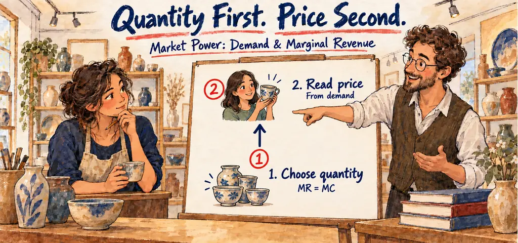
Quantity comes from MR. Price comes from demand.

Draw downward demand and a steeper MR below it, then rising MC. The MR-MC intersection gives monopoly quantity. Move vertically to demand for price. The efficient quantity lies where demand meets MC, so the units between monopoly and efficient quantity generate deadweight loss.

For monopolistic competition, add ATC. Short-run analysis looks like monopoly. Long-run entry shifts demand until it is tangent to ATC. Price equals ATC, but demand’s tangency occurs left of minimum ATC.

A firm with market power faces a downward-sloping demand curve. To sell more output, it must generally lower price, so marginal revenue lies below price. For a linear demand curve, MR shares the vertical intercept and falls twice as fast, but this shortcut does not apply mechanically to every nonlinear demand schedule.

Use a two-step procedure. First find the quantity where MR equals rising MC. Second move vertically from that quantity to demand to find the highest price consumers will pay. Reading price from the MR curve is a classic distractor because MR selects quantity but is not the price charged.

Quantity first, price second

MR equals MC at 40 units. Demand at 40 units shows a price of $30, while ATC is $22. The firm charges $30, earns (30-22)(40)=$320, and does not charge the lower MR value. If demand meets MC at 55 units, monopoly’s restriction from 55 to 40 creates deadweight loss.

Use elasticity as a diagnostic after locating the monopoly choice. With nonnegative marginal cost, an output on the inelastic segment cannot maximize profit: a small output reduction would increase revenue while also avoiding production cost. Therefore the chosen point must be on the elastic segment, except for the zero-MC boundary case at unit elasticity.

Price discrimination changes the revenue logic. If a firm can charge different buyers according to willingness to pay and prevent resale, it may expand output. Perfect first-degree discrimination converts consumer surplus into producer surplus and produces the efficient quantity where demand meets MC in the basic model. It does not eliminate market power. It changes distribution and output.

Monopolistic competition uses the same short-run demand-MR-MC method, but free entry shifts each firm’s demand left and makes it more elastic until it is tangent to ATC. Long-run economic profit is zero, yet price exceeds MC and output is below the ATC-minimizing scale. This is excess capacity, not a short-run shutdown signal.

For oligopoly, one-firm curves may be insufficient because each firm’s payoff depends on rivals’ choices. A payoff matrix, best-response analysis, or kinked-demand story may replace the simple monopoly graph. Always identify the market structure before applying a picture. Downward demand alone does not prove pure monopoly. Many differentiated sellers face downward demand.

Cost changes have precise effects. A lower fixed cost shifts ATC downward but leaves MC, monopoly quantity, and monopoly price unchanged in the short run. Profit rises. A lower marginal cost shifts MC downward, usually increasing quantity and lowering price. A demand increase shifts demand and MR, changing both quantity and price. These comparative-static patterns are stronger than vague claims that “lower cost always lowers price.”