A competitive firm requires a separate market graph

Transfer price, not total market quantity.

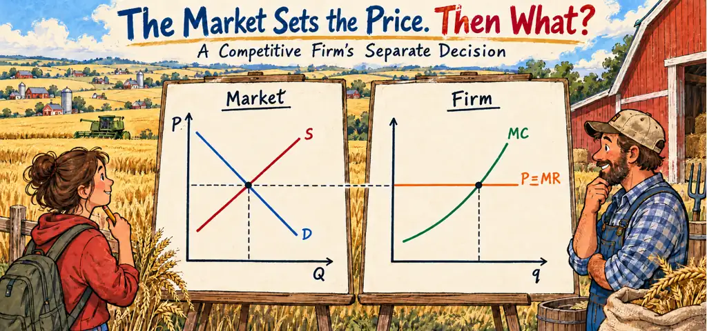
Market supply and demand determine price. On the firm graph, cost or revenue appears vertically and firm output horizontally. The transferred price becomes horizontal P=MR. Add rising MC and U-shaped AVC and ATC. Price’s intersection with MC gives output. Its relation to AVC determines operation. Its relation to ATC determines profit.

The firm graph can show a profit rectangle, loss rectangle, shutdown point, or long-run zero-profit tangency. Keep the market’s uppercase Q and firm’s lowercase q distinct in scratch work.

Perfect competition operates at two levels. The industry graph contains market demand and market supply and determines the equilibrium price. The individual firm is too small to affect that price, so it faces a horizontal demand curve at the market price. Combining both levels on one set of axes produces conceptual mistakes even if the curves look familiar.

On the firm graph, label output q horizontally and dollars per unit vertically. Draw P=MR=D horizontally, rising MC, U-shaped AVC, and U-shaped ATC above AVC. The firm chooses the quantity where price equals the rising portion of MC. That is an output decision. Profit requires comparing price with ATC at that quantity.

Transfer only the price

Market equilibrium is $18 at 50,000 units. The representative firm’s MC reaches $18 at 120 units and its ATC there is $15. The firm produces 120, not 50,000, and earns (18-15)(120)=$360. The market quantity is divided among all firms.

Positive profit attracts entry in the long run. Market supply shifts right, price falls, and each existing firm’s output adjusts along MC until price is tangent to minimum ATC in the constant-cost model. Loss causes exit and the reverse supply shift. Zero economic profit includes a normal return to the owner’s resources, so firms have no incentive to enter or leave.

A change in fixed cost shifts AFC and ATC but not AVC or MC. Therefore it does not change a continuing firm’s short-run profit-maximizing output, though it changes profit and can influence long-run entry or exit. A variable input-price change shifts AVC, ATC, and MC and can change output immediately.

Keep notation disciplined: uppercase Q for the market, lowercase q for one firm. An industry’s short-run supply is the horizontal sum of firms’ MC portions above AVC, not one firm’s curve copied onto the market graph. The visual separation is not decoration. It represents price formation at one level and price-taking optimization at another.

Shifts must also be assigned to the proper panel. Stronger consumer demand shifts market demand, raises market price in the short run, and moves the firm’s horizontal price line upward. It does not directly shift the firm’s MC. A cheaper production input can shift every firm’s MC and the industry supply curve. Describing both panels in sequence-market event, new price, firm response-turns a two-graph question into three manageable steps.