Chi-Square Tests in Genetics: Calculation and Examples
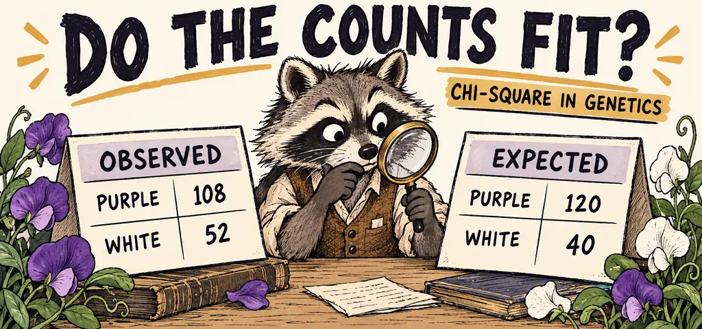
A chi-square goodness-of-fit test compares observed offspring counts with counts predicted by a specified inheritance model. Calculate expected counts, add the squared deviations divided by their expectations, then use the appropriate degrees of freedom. A result that fails to reject the model does not prove it correct.
Suppose you flip a fair coin a hundred times. Fifty heads would fit your expectation, and forty-six or fifty-three would hardly be surprising. Seventy-one heads would make you question the model. How much deviation should count as evidence? A chi-square test compares the observed counts with a stated prediction while accounting for sample size, which makes it useful for offspring counts as well as coin flips.
Watch the process
Chi-squared Test
Real offspring counts can match a predicted ratio exactly, but sampling often produces deviations. A \(Bb \times Bb\) cross that yields 78 purple and 22 white has not produced 3:1, a chi-square calculation determines whether that deviation is significant at the chosen level. A cross yielding 60 purple and 40 white is a different matter. Between those two cases is a line, and chi-square goodness-of-fit is the procedure that draws it. Its formula appears on the AP Biology equation sheet.
The Null Hypothesis Comes First
Every chi-square test begins with a null hypothesis: a specific quantitative model for the population probabilities being tested. Sampling variation explains deviations under that model, provided the test assumptions hold. In genetics the null hypothesis is normally a named ratio. “The offspring fit a 3:1 phenotypic ratio, and the deviation from it is due to random sampling” is a null hypothesis. “The genes are linked” alone is too vague for this goodness-of-fit calculation. A linkage model with a specified recombination frequency could supply testable expected counts.
The statistic itself compares observed counts to expected counts, class by class: \[\chi^{2} = \sum \frac{(o-e)^{2}}{e}\] where \(o\) is the observed count in a phenotypic class, \(e\) is the count that class is expected to contain under the null hypothesis, and the sum runs over every class. Three details keep the calculation valid. Use raw counts, never percentages or fractions. Compute expected counts by multiplying the total number of offspring by each class’s fraction of the ratio. And square the difference before dividing, so that deviations in either direction add rather than cancel.
For a fully specified ratio with no parameters estimated from these offspring counts, degrees of freedom is the number of classes minus one, where a phenotypic class is one of the distinct appearances the offspring were sorted into, purple and white are two classes; round yellow, round green, wrinkled yellow, and wrinkled green are four. For a 3:1 test there are two classes and \(df = 1\). For a 9:3:3:1 test there are four classes and \(df = 3\). The subtraction reflects the fixed total: once all but one class count are known, the last is determined. Estimating model parameters from the same data can require additional adjustments. Use independent observations, mutually exclusive categories, and sufficiently large expected counts (the examples here use at least five per class).
Reading the Table
The exam supplies critical values. Find the column for your degrees of freedom, read the value in the \(p = 0.05\) row, and compare it with your calculated \(\chi^{2}\). Before you use it, understand what the number in that row means. The p-value is the probability of getting a deviation at least as large as the one you observed if the null hypothesis is true. The critical value is the \(\chi^{2}\) that corresponds to \(p = 0.05\): cross it and your result falls into the most extreme five percent of outcomes that chance alone would produce. Biologists use 0.05 by convention, not by discovery. It is a threshold chosen to limit the long-run false-rejection rate under the null model, use the significance level supplied for the test.
Notice how the values rise across the row: 3.84 at \(df = 1\), 7.81 at \(df = 3\), 15.51 at \(df = 8\). More classes means more places for deviation to appear, so a larger statistic is required to reject the model at the same significance level. Never compare a \(\chi^{2}\) to a threshold you remember from a different problem.
| Degrees of freedom | 1 | 2 | 3 | 4 | 5 | 6 | 7 | 8 |
|---|---|---|---|---|---|---|---|---|
| Critical value, \(p = 0.05\) | 3.84 | 5.99 | 7.81 | 9.49 | 11.07 | 12.59 | 14.07 | 15.51 |
The decision rule has exactly two branches, and the wording matters as much as the arithmetic. If \(\chi^{2}\) meets or exceeds the critical value, reject the null hypothesis: a deviation at least this large has a probability at most 0.05 under the null model, giving evidence against the null model, not proof that chance was impossible. If \(\chi^{2}\) is below the critical value, fail to reject the null hypothesis: the data are consistent with the predicted ratio. For an AP conclusion, write “fail to reject” rather than claiming the null is proven. If rounding places a result exactly on the boundary, use the precision or decision rule provided. Failing to reject means the data give you no reason to abandon the model, which is a weaker and more honest claim.
Worked Chi-Square 1: Testing a 3:1 Monohybrid Ratio
Two heterozygous purple-flowered plants are crossed. Of 160 offspring, 108 are purple and 52 are white. Test the hypothesis that these data fit the 3:1 ratio predicted for a monohybrid cross with complete dominance.
Null hypothesis. The offspring fit a 3:1 purple-to-white ratio, and any deviation is due to chance.
Expected counts. Purple is \(\tfrac{3}{4}\) of the ratio and white is \(\tfrac{1}{4}\), so with 160 offspring the expectations are \(\tfrac{3}{4}(160) = 120\) purple and \(\tfrac{1}{4}(160) = 40\) white. The expected counts must sum to the observed total, and \(120 + 40 = 160\) confirms the setup.
| Class | \(o\) | \(e\) | \(o-e\) | \((o-e)^{2}\) | \((o-e)^{2}/e\) |
|---|---|---|---|---|---|
| Purple | 108 | 120 | \(-12\) | 144 | 1.20 |
| White | 52 | 40 | \(+12\) | 144 | 3.60 |
| Total | 160 | 160 | 4.80 |
Statistic and degrees of freedom. \(\chi^{2} = 1.20 + 3.60 = 4.80\). There are two classes, so \(df = 2-1 = 1\).
Comparison. The critical value at \(df = 1\) and \(p = 0.05\) is 3.84. Since \(4.80 > 3.84\), the deviation is larger than chance comfortably explains. Notice that the white class contributed three times as much to the statistic as the purple class did, even though both deviated by 12 offspring. Dividing by \(e\) makes the same absolute deviation matter more in a small class.
Answer
\(\chi^{2} = 4.80\) exceeds the critical value of 3.84 at \(df = 1\), so we reject the null hypothesis. The offspring do not fit a 3:1 ratio, and possible explanations such as unequal genotype viability or scoring bias deserve investigation. This result does not identify which assumption failed, and a false rejection remains possible.
Worked Chi-Square 2: Testing a 9:3:3:1 Dihybrid Ratio
A dihybrid cross of pea plants heterozygous for seed shape and seed color yields 320 offspring: 190 round yellow, 58 round green, 54 wrinkled yellow, and 18 wrinkled green. Do the data support independent assortment of the two genes?
Null hypothesis. The two genes assort independently, so the offspring fit a 9:3:3:1 ratio, and any deviation is due to chance.
Expected counts. The four fractions are \(\tfrac{9}{16}\), \(\tfrac{3}{16}\), \(\tfrac{3}{16}\), and \(\tfrac{1}{16}\). With 320 offspring, one-sixteenth is 20, so the expectations are \(9(20) = 180\), \(3(20) = 60\), \(3(20) = 60\), and \(1(20) = 20\). Converting the ratio to sixteenths first, then scaling, is faster and less error-prone than four separate multiplications.
| Class | \(o\) | \(e\) | \(o-e\) | \((o-e)^{2}\) | \((o-e)^{2}/e\) |
|---|---|---|---|---|---|
| Round yellow | 190 | 180 | \(+10\) | 100 | 0.56 |
| Round green | 58 | 60 | \(-2\) | 4 | 0.07 |
| Wrinkled yellow | 54 | 60 | \(-6\) | 36 | 0.60 |
| Wrinkled green | 18 | 20 | \(-2\) | 4 | 0.20 |
| Total | 320 | 320 | 1.43 |
Statistic and degrees of freedom. \(\chi^{2} = 0.56 + 0.07 + 0.60 + 0.20 = 1.43\). There are four classes, so \(df = 4-1 = 3\).
Comparison. The critical value at \(df = 3\) and \(p = 0.05\) is 7.81. The calculated value is far below it, so the data do not provide sufficient evidence to reject the stated model at the 0.05 level.
Interpreting the result
\(\chi^{2} = 1.43\) is less than the critical value of 7.81 at \(df = 3\), so we fail to reject the null hypothesis. The data are consistent with a 9:3:3:1 ratio and therefore with independent assortment of the two genes. This does not prove independence; it means the counts give no reason to abandon that model.
A Test Cross Scored Against 1:1
A test cross between a heterozygous parent and a homozygous recessive partner produces 88 offspring: 51 showing the dominant phenotype and 37 showing the recessive one. Test the 1:1 prediction.
The null hypothesis is that the offspring fit 1:1 and the deviation is due to chance. Two classes at \(\tfrac{1}{2}\) each, so both expected counts are \(\tfrac{1}{2}(88) = 44\). The deviations are \(51-44 = +7\) and \(37-44 =-7\). Square each: \(49\). Divide each by its expected count: \(49/44 \approx 1.1136\). Both classes have the same expected count here, so both contribute the same amount. \[\chi^{2} = 2(49/44) \approx 2.23, \qquad df = 2-1 = 1.\] The critical value at \(df = 1\) is 3.84, and \(2.23 < 3.84\).
Answer
Fail to reject. A split of 51 to 37 out of 88 is well within what random sampling produces from a true 1:1 ratio, so these data give no reason to doubt that the dominant-looking parent was heterozygous.
Chi-square converts a gap between observed and expected counts into one number you can compare against a published threshold.
Nothing about the biology changes; what changes is that a judgment call becomes a decision rule.
Do not put percentages, fractions, or ratios into the formula. Only raw counts go in, because the size of the sample is exactly the information the test needs.
Use Expected Counts and Interpret the Test
The denominator is the expected count, so each contribution is \((o-e)^2/e\). Dividing by the observed count changes the statistic, even if the numerical difference is small when the counts are close. You are asking how big the deviation is relative to what the model predicted, so the model’s number belongs underneath. A deviation of 12 is trivial against an expectation of 1,200 and alarming against an expectation of 20.
Failing to reject a hypothesis does not prove it. Rejecting the null hypothesis says the data are unlikely under the proposed model, which is evidence against that model. Failing to reject says the data are compatible with the model, which is not evidence that the model is right, a small sample can have too little power to distinguish competing models. State whether you reject or fail to reject the null hypothesis; neither outcome proves a model.
Count the phenotypic classes when choosing degrees of freedom. For a fully specified ratio with no parameters estimated from the offspring data, subtract one from that count. A four-class dihybrid test has \(df = 3\). Increasing the sample size does not change that value, but it can improve the expected counts: a sample of 32 gives only two expected offspring in the smallest class of a 9:3:3:1 ratio and fails the usual expected-count guideline.
Chi-square goodness of fit
Practice question 1
A student tests offspring counts against a 9:3:3:1 ratio. The correct number of degrees of freedom is
-
1
-
2
-
3
-
4
Practice question 2
A monohybrid cross produces 400 offspring and the null hypothesis is a 3:1 ratio. The expected counts are
-
200 dominant and 200 recessive
-
300 dominant and 100 recessive
-
250 dominant and 150 recessive
-
100 dominant and 300 recessive
Practice question 3
A test of a 3:1 ratio gives \(\chi^{2} = 2.10\), and the critical value at \(p = 0.05\) is 3.84. The correct conclusion is that
-
the null hypothesis is rejected, because the observed counts differed from the expected counts
-
the null hypothesis is not rejected, and the data are consistent with a 3:1 ratio
-
the null hypothesis is proven correct, since the statistic is small
-
the null hypothesis is rejected, because the statistic is smaller than the critical value
Practice answer key
1. C; 2. B; 3. B.
Practice answer explanations
-
Chi-square goodness of fit, Question 1. Choice C is correct. Degrees of freedom is the number of phenotypic classes minus one, and a 9:3:3:1 ratio has four classes, so \(df = 3\). Choice A would be right for a two-class test such as 3:1. Choice B subtracts two instead of one. Choice D forgets to subtract at all.
-
Chi-square goodness of fit, Question 2. Choice B is correct. Expected counts are the total multiplied by each class’s fraction: \(\tfrac{3}{4}(400) = 300\) and \(\tfrac{1}{4}(400) = 100\). Choice A splits the offspring evenly, which is the expectation for a 1:1 ratio. Choice C uses a 5:3 split that matches no Mendelian prediction. Choice D reverses the two classes, assigning the larger count to the recessive class.
-
Chi-square goodness of fit, Question 3. Choice B is correct. A calculated value below the critical value means a deviation at least this large has a probability above 0.05 under the null model, so the null hypothesis is not rejected and the data remain consistent with 3:1. Choice A rejects on the mere existence of a deviation, which can occur even when the model is correct. Choice C claims proof, and a failure to reject never proves a null hypothesis. Choice D runs the decision rule backwards, rejecting when the statistic falls below the threshold instead of above it.
Continue your review at the AP Biology study hub.

Related to This Article
More math articles
- Innovative Forecasts: Population Models are Predicting the Future
- Environmental Chemistry: Carbon, Water and Nutrients
- How to Graph an Equation in the Standard Form?
- The Best Grade 3 ELA Practice Tests for Montana Students
- The Ultimate 7th Grade NDSA Math Course (+FREE Worksheets)
- Grade 4 Math Flashcards (Free Online: Formulas, Terms & Concepts)
- Free Grade 3 Math PDFs for Kentucky KSA: 49 Single-Skill Worksheets with Step-by-Step Keys
- How to Write Two-variable Inequalities Word Problems?
- Balancing Probabilities: A Comprehensive Guide to the Expected Value of Random Variables
- 3rd Grade NDSA Math Worksheets: FREE & Printable









What people say about "Chi-Square Tests in Genetics: Worked Examples"?
No one replied yet.