Social and factor graphs require the correct marginal curves
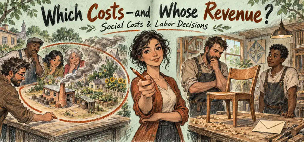
Social and factor graphs require the correct marginal curves: this Effortless Math guide explains the topic in plain language, shows how it works through solved examples, and gives you free practice to try immediately, so the idea sticks instead of staying abstract.
Private versus social values and wage versus marginal revenue product answer different questions.
The diagram shows a negative production externality. Which relationship explains why the market quantity exceeds the efficient quantity?
- Marginal social cost lies below supply.
- Marginal social benefit lies above demand.
- Demand shifts right of social benefit.
- Private marginal cost lies above social marginal cost.
- Marginal social cost lies above private marginal cost.
Marginal social cost lies above private marginal cost. External production damage makes social marginal cost exceed the private cost represented by ordinary supply.
On a monopsony labor graph, which curves determine employment, and which curve then determines the wage?
- Labor supply and MRP determine employment, then MRC gives wage
- MRP and MRC determine employment, then labor supply gives wage
- Labor supply and MRC determine both values
- Product demand determines employment, then MRP gives wage
- Average product determines employment, then ATC gives wage
MRP and MRC determine employment, then labor supply gives wage The monopsonist hires where the added revenue from labor equals the added cost of hiring labor. After finding that employment level, move down to the labor-supply curve to read the wage.
In a competitive labor market, the market wage is $24 per hour. How does one price-taking employer choose labor?
- Hire where MRP equals the $24-per-hour wage
- Hire where average product equals $24
- Set the wage where market labor demand meets market labor supply
- Hire where MRC lies above labor supply
- Choose employment at minimum ATC
Hire where MRP equals the $24-per-hour wage The market graph sets the wage. For one competitive employer, marginal resource cost is the constant $24 wage, so the firm’s hiring point is where its downward-sloping MRP curve reaches $24 per hour.
Watch the idea in action
A focused video lesson from Axel Abrica.
For a negative production externality, market supply is MPC and social cost MSC lies above it. Market quantity occurs where demand meets MPC. Efficient quantity where MSB meets MSC. For a positive consumption externality, MSB lies above private demand.
Rebuild a graph from one sentence
“A binding ceiling is imposed below equilibrium.” Draw supply and demand, mark their intersection, and place the ceiling below it. At that legal price, read quantity supplied from supply and quantity demanded from demand. The horizontal distance is the shortage. This construction is safer than trying to recall a finished picture because every feature follows from the sentence.
Describe the graph in one sentence
After drawing, say: “The event shifts ___ because ___, so equilibrium ___ and ___.” If you cannot complete the mechanism, the picture is not yet reliable.
Advanced-looking diagrams become manageable when every curve is translated into a marginal sentence. An externality graph asks whether private buyers and sellers face all costs and benefits. A factor graph asks how much revenue another input creates and what hiring it costs. The drawing follows those meanings.
For negative production externalities, ordinary supply is marginal private cost and MSC lies above it by marginal external cost. The market chooses where demand or MSB meets MPC. Society prefers where MSB meets MSC. For positive consumption spillovers, ordinary demand is MPB and MSB lies above it. The direction of inefficiency follows from the omitted value, not from a memorized curve color.
Place the missing curve
A factory’s next unit costs it $14 and causes $6 of external damage. At that quantity, MSC is $20. If buyers’ marginal benefit is $17, the unit is privately worthwhile but socially wasteful. The social-cost curve must lie above private supply, and efficient output is lower than market output.
In a competitive labor market, downward labor demand represents MRP and upward labor supply represents workers’ opportunity cost. Their intersection determines wage and employment. One competitive firm takes the wage as given and hires until its MRP equals that wage. A change in product demand can shift labor demand because it changes the revenue created by workers.
The curves should not be mixed. A competitive wage comes from market labor supply and demand. Private supply is not MSC with pollution. Market demand is not MSB when consumer benefits spill over. A correct label can be more important than the curve’s artistic shape.
Use a five-part audit: identify the chooser, label the vertical unit, state what each marginal curve includes, find the decision intersection, and then locate any price or wage on the appropriate nonmarginal curve. This method handles unfamiliar graphs because it rebuilds them from incentives rather than recalling a snapshot.
Six-graph closed-book drill
On six blank sets of axes, rebuild: market supply and demand after one shift. A per-unit tax wedge. A competitive firm with profit or loss. A single-price monopoly. A negative externality. And a competitive labor market. For each drawing, label both axes, every curve, the original decision, the changed decision, and one sentence explaining the mechanism. Check the book only after all six are complete.

Reza is an experienced Math instructor and a test-prep expert who has been tutoring students since 2008. He has helped many students raise their standardized test scores--and attend the colleges of their dreams. He works with students individually and in group settings, he tutors both live and online Math courses and the Math portion of standardized tests. He provides an individualized custom learning plan and the personalized attention that makes a difference in how students view math.
Related to This Article
More math articles
- 7th Grade STAAR Math Practice Test Questions
- Pre-Algebra Survival Guide: Everything You Need to Pass in 2026
- Limits on judicial power
- Geometry in Action: Crafting the Circumscribed Circle of a Triangle
- What Are the 5 Ways to Prove Congruence?
- Descriptive Statistics Calculator — Mean, SD, Quartiles (Free)
- 5th Grade MCAP Math Worksheets: FREE & Printable
- How to Use Expanded Form to Multiply One-Digit Numbers By 3-digit or 4-digit Numbers
- How to Solve Word Problems of Counting Bills and Coins
- Algebra Puzzle – Challenge 55





















What people say about "Social and Factor Graphs Need the Right Curves"?
No one replied yet.