AP Business with Personal Finance: Break-Even Analysis Step by Step (2027 Prep)

A bookmark stall collects $360 after selling forty kits at $9 each. Then its owner checks the costs. With $245 of fixed costs and $3 of variable cost per kit, the stall has lost $5.
One more kit changes the result. Selling forty-one brings revenue to $369 and total modeled costs to $368, leaving $1. Those two sales levels help explain why a calculated break-even quantity sometimes needs rounding up.
For AP Business with Personal Finance, start with the period and cost assumptions, then calculate what each sale contributes toward fixed costs. The fictional stall below keeps the same numbers through the calculation, graph and changed conditions, so you can check every conclusion against its costs.
Connect the example to the course framework
College Board's current course and exam description covers fixed and variable expenses in Topic 3.4. Topic 3.5 includes calculating how many goods or services a business needs to sell in a period to cover its costs. Our teaching model uses one product.
The model is simplified. The quantities and prices are invented, and the result is an explanation of its assumptions rather than advice to start a stall or charge a particular price.
Use the AP Business with Personal Finance Online Center to organize your wider course review after working through the example. Here, keep your attention on the difference between sales revenue and the costs that those sales must cover.
Put every cost in the same period
Our base case covers one weekend event. Fixed costs are $245 for that event, and remain unchanged across the base model's range of zero to sixty kits. Each kit sold has $3 of variable cost, including the materials and packaging specified in this example.
Keep the units visible. The $245 is dollars per event, while the $3 is dollars per kit. Multiplying $3 by the number of kits sold gives total variable cost for the event.
All kits produced for this model are sold, and the selling price stays at $9. These are all the model's stated costs. A real cost estimate would need to check its own omissions, including labor and fees, before using the same calculation.
The OpenStax break-even chapter explains the assumptions behind this kind of cost-volume-profit analysis. The fixed-cost range matters because a business may need a different cost model when its activity passes a capacity limit.
Find contribution before dividing fixed costs
Each $9 sale has $3 of variable cost attached to it. Subtracting that cost leaves a $6 contribution margin per kit, which is available to cover the event's fixed costs and then contribute to modeled profit.
Subtract first. The calculation is $9 – $3 = $6 per kit. Dividing $245 by the full $9 selling price would ignore the variable cost that accompanies every sale.
The quantity needed at the exact break-even point is fixed costs divided by contribution margin per unit. For this stall, $245 / $6 = 40.833333… kits. The fractional quantity is the intersection in a continuous model, where revenue equals total cost.
Whole kits need a further interpretation. The smallest whole number of kits with no modeled loss is forty-one, because forty kits still leave $5 of fixed costs uncovered. Forty-one produces a small positive result, rather than exactly zero profit.
Check the answer using revenue and total cost
At forty kits, revenue is 40 x $9 = $360. Variable cost is 40 x $3 = $120, and total cost is $245 + $120 = $365. Revenue minus total cost gives a $5 loss.
Check forty-one too. Revenue is 41 x $9 = $369, variable cost is $123, and total cost is $368. The difference is a $1 profit within this model.
The two results bracket the exact intersection. Rounding down to forty would leave a loss, so it cannot satisfy a requirement to cover the fixed event costs and the cost of every kit sold.
In a written explanation, state whether you are reporting the exact mathematical intersection or the smallest feasible whole-unit quantity with no loss. Keeping that distinction explicit is more useful than writing a rounded number without its meaning.
Read the graph alongside the calculation
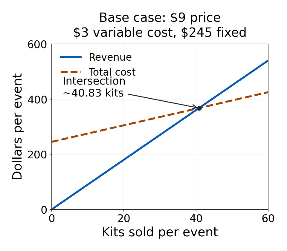
Let q be kits sold. Base-case revenue is 9q dollars and total cost is 245 + 3q dollars, leaving a modeled profit or loss of 6q – 245 dollars.
The graph uses those equations. Revenue starts at zero, while total cost starts at $245 because the fixed event costs remain even when no kits sell. The intersection lies between forty and forty-one kits, matching the calculation above.
The base-case graph data (CSV) contains every whole-kit quantity from zero through sixty with its revenue, total cost and profit or loss. Use the displayed sample table to check a few points, then plot additional rows if you want to reconstruct the graph yourself.
| Kits sold | Revenue ($) | Total cost ($) | Profit/loss ($) |
|---|---|---|---|
| 0 | 0 | 245 | -245 |
| 20 | 180 | 305 | -125 |
| 40 | 360 | 365 | -5 |
| 41 | 369 | 368 | 1 |
| 50 | 450 | 395 | 55 |
Change the price and keep the comparison conditional
Now consider a separate price scenario. The selling price becomes $10 per kit, while variable cost remains $3 and fixed event costs remain $245 over the same zero-to-sixty range.
Recalculate contribution. It is now $7 per kit, so the exact break-even quantity is $245 / $7 = 35 kits. Revenue and total cost both equal $350.
The changed calculation does not predict demand. It shows how the threshold changes under the new assumptions, while the number of customers willing to pay $10 still needs evidence. Comparing the prices requires both the cost calculation and a defensible expectation about sales at each price.
Return to the base $9 scenario when reading the next section. Keeping the scenarios separate prevents a price change from slipping into a calculation that was meant to investigate capacity alone.
Recheck a cost change above forty kits
Suppose a different event setup now has a capacity condition. Fixed costs are $245 for zero through forty kits, but selling forty-one through eighty requires an extra $60 equipment rental. The selling price stays at $9 and variable cost stays at $3 per kit.
Use the applicable range. Above forty kits, fixed costs become $305, so the old forty-one-kit result no longer applies. At forty-one, revenue is still $369, but total cost is $305 + $123 = $428, leaving a $59 loss.
For the higher range, divide $305 by the unchanged $6 contribution. That gives 50.833333… kits, making fifty-one the smallest whole quantity with no loss in this changed scenario. Fifty kits lose $5, while fifty-one produces $1 of modeled profit.
Check both ranges. The lower range ends at forty kits and never covers the original $245 fixed costs, so it provides no earlier no-loss quantity. Fifty-one lies within the stated forty-one-to-eighty range, making it consistent with the cost assumptions used to calculate it.
This capacity example extends the base teaching model. It illustrates an assumption check and makes no prediction that this particular step-cost scenario will appear on an AP exam.
Recognize when the simple division stops helping
If the selling price equals variable cost, each sale contributes zero toward positive fixed costs. Dividing by zero cannot provide a finite break-even quantity. With a price below variable cost, additional sales make the modeled loss larger while fixed costs remain positive.
Inspect a negative answer. It does not mean that a business can sell a negative quantity and cover its costs. Revisit the contribution margin and explain why the stated model cannot reach break-even through positive sales.
A stall selling different products also needs care. The $6 contribution belongs to this kit alone, so it cannot automatically be applied to a mixture of bookmarks and other goods with different prices or costs.
Build your own calculation record
The blank break-even calculation record (CSV) gives you space to name the period and applicable capacity range before entering price, variable cost and fixed costs. Record the exact intersection separately from the whole-unit interpretation, then verify the result using revenue and total cost.
Begin with the base case. Compare forty and forty-one kits, and use the graph data to explain the remaining loss and the small positive result in complete sentences.
Continue in the AP Business with Personal Finance Online Center when you are ready to review another business-finance topic. Keep your course or project assumptions attached to your calculation, so another reader can see which costs and sales conditions your answer actually uses.
2027 preparation edition. Current College Board framework and clarifications checked October 11, 2026. Bookmark stall, prices, quantities, graph and changed scenarios are original fictional teaching material, not official or recalled exam questions or a real business forecast. Profit/loss refers only to the explicitly modeled costs. The cover balance is a conceptual illustration, not a numerical chart.

Related to This Article
More math articles
- How to Solve Angle Measurements Word Problems
- The Harlem Renaissance and Garveyism
- Full-Length GED Math Practice Test-Answers and Explanations
- The Best Calculator for the SAT or ACT
- Idaho ISAT Grade 8 Math Free Worksheets: 72 Free PDF Worksheets, One Skill at a Time
- SAT Vs PSAT Tests
- 4th Grade RISE Math Worksheets: FREE & Printable
- Microorganisms
- 10 Most Common 7th Grade MAP Math Questions
- How to Add and Subtract Integers: Word Problems






What people say about "AP Business with Personal Finance: Break-Even Analysis Step by Step (2027 Prep)"?
No one replied yet.