Long-run average cost envelopes possible plants
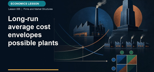
Long-run average cost envelopes possible plants: this Effortless Math guide explains the topic in plain language, shows how it works through solved examples, and gives you free practice to try immediately, so the idea sticks instead of staying abstract.
The firm chooses a plant and an operating point.
Each short-run ATC curve belongs to a particular plant size. Long-run average cost shows the lowest attainable average cost for each output when the firm can choose among plants. The firm need not operate every plant at its own minimum. It chooses the plant that minimizes cost for the intended output.
Imagine three kitchens: small, medium, and large. At low output, the small kitchen may have the lowest average cost because the larger spaces carry unused capacity. At medium output, crowding raises the small kitchen’s cost and the medium plant becomes cheaper. At high output, the large kitchen may be least costly. LRAC traces the lowest available point across all plant choices.
The envelope is a planning curve. Once the firm builds a particular plant, it operates on that plant’s short-run ATC until it can adjust capacity again. A firm expecting 500 units chooses a different plant than one expecting 5,000. Movement along LRAC therefore combines a change in output with an optimal change in all relevant inputs.
Economies of scale occur when output grows more than proportionally to all inputs and long-run average cost falls. Specialization, indivisible equipment, and spreading design or network costs can create them. Constant returns to scale mean output changes in the same proportion as inputs. Diseconomies of scale arise when coordination, communication, and monitoring problems make output grow less than proportionally, raising LRAC.
Returns to scale describes a physical experiment: change every input by the same percentage and observe output. Economies of scale describes the associated cost result as the firm adjusts all inputs optimally. In the standard setting they point in corresponding directions, but keep the language clear: one compares inputs with output. The other compares output with long-run average cost.
If all inputs rise 50 percent and output rises 80 percent, the firm has increasing returns to scale over that range. Constant returns would raise output 50 percent, not double it. This proportional comparison differs from marginal product, which changes one input.
| All inputs rise 50% | Output response | Cost interpretation |
|---|---|---|
| More than 50% | Increasing returns | LRAC tends to fall |
| Exactly 50% | Constant returns | LRAC tends to be constant |
| Less than 50% | Decreasing returns | LRAC tends to rise |
Increasing returns can result from specialization and indivisible capital. A large machine may be too costly for small output but efficient when used heavily. Diseconomies can arise when information must pass through more managerial layers or when local decisions become harder to coordinate. These are long-run scale mechanisms, not short-run crowding around a fixed oven.
Two experiments, two concepts
Holding a factory fixed, adding workers eventually lowers MP: diminishing marginal returns. Building a larger factory while increasing labor, machines, and space 40 percent raises output 60 percent: increasing returns to scale. Both can be true because the first changes one input and the second changes all inputs.
Minimum efficient scale is the smallest output at which long-run average cost reaches its lowest sustainable level. If it is small relative to market demand, many firms can operate efficiently. If it is large relative to demand, one or a few firms may serve the market at lower cost, contributing to natural monopoly or oligopoly.
On the exam, underline “all inputs” or “one variable input.” Then compare percentages rather than raw amounts. A 20-unit output increase is not enough to classify returns without knowing the initial output and input changes.
A firm doubles labor and capital, and output exactly doubles. The firm exhibits
- economies of scale
- constant returns to scale
- diseconomies of scale
- diminishing marginal product
- increasing marginal cost by definition
constant returns to scale When all inputs and output change in the same proportion, production has constant returns to scale.
The long-run average-cost curve is called an envelope because it
- equals marginal cost for every possible plant
- contains only costs that remain fixed in the long run
- joins the lowest-cost points available across plant sizes
- traces the highest short-run average cost at each output
- must be horizontal when every input is variable
joins the lowest-cost points available across plant sizes For each output, the long-run curve selects the least costly point available from all short-run plant curves.
Watch the idea in action
A focused video lesson from MIT OpenCourseWare.

Reza is an experienced Math instructor and a test-prep expert who has been tutoring students since 2008. He has helped many students raise their standardized test scores--and attend the colleges of their dreams. He works with students individually and in group settings, he tutors both live and online Math courses and the Math portion of standardized tests. He provides an individualized custom learning plan and the personalized attention that makes a difference in how students view math.
Related to This Article
More math articles
- How to Add and Subtract Complex Numbers? (+FREE Worksheet!)
- The Best Grade 4 Math Book for Hawaii Students
- 3rd Grade SBAC Math FREE Sample Practice Questions
- Top 10 TSI Math Practice Questions
- Is the ACCUPLACER Test hard?
- Top 10 Tips You MUST Know to Retake the ACCUPLACER Math
- Grade 5 Literary Analysis: Theme, Character Change, and Text Evidence Made Practical
- Percent of Change Practice — Increase & Decrease (Free)
- PSAT/NMSQT Math Flashcards (Free Online: Formulas, Terms & Concepts)
- Symbolic Interactionism





















What people say about "Long-Run Average Cost as an Envelope"?
No one replied yet.