Single-price monopoly creates underproduction
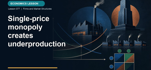
Single-price monopoly creates underproduction: this Effortless Math guide explains the topic in plain language, shows how it works through solved examples, and gives you free practice to try immediately, so the idea sticks instead of staying abstract.
The efficient units between the monopoly quantity and the efficient quantity are not sold.
Relative to the efficient output, a single-price monopoly stops production where
- marginal benefit is below marginal cost
- marginal benefit still exceeds marginal cost
- price equals marginal cost
- consumer surplus is maximized
- average total cost is minimized
marginal benefit still exceeds marginal cost The monopoly quantity is below the P=MC quantity, so excluded units have willingness to pay above marginal cost.
Compared with a competitive market with the same demand and cost, a single-price monopoly generally produces
- less output at a higher price
- more output at a lower price
- the efficient output at a higher price
- the same output at the same price
- less output at a lower price
less output at a higher price Because monopoly chooses where MR=MC rather than P=MC, it restricts output and raises price relative to competition.
Watch the idea in action
A focused video lesson from Economics in Many Lessons.
The efficient quantity occurs where demand, representing marginal benefit, meets MC. Monopoly instead uses MR=MC, producing less and charging more. For the missing units, willingness to pay exceeds marginal cost, so their unrealized gains form deadweight loss. Monopoly profit is largely a transfer from consumer surplus. The deadweight-loss triangle is the net social loss in the basic model.
Compare two intersections on the same graph. Q_m comes from MR and MC and determines the single-price monopoly outcome. Q_e comes from demand and MC because efficiency compares marginal benefit with marginal cost. Since MR lies below demand, Q_m<Q_e when MC is ordinary and positive.
At units between Q_m and Q_e, demand lies above MC. Buyers value each unit more than the resources needed to produce it, but the single-price policy withholds it. The area between demand and MC over that interval is deadweight loss. It is not the entire monopoly profit rectangle.
| Benchmark | Equality | Meaning |
|---|---|---|
| Monopoly quantity | MR=MC |
Maximizes seller profit |
| Efficient quantity | P=MB=MC |
Maximizes total surplus |
| Monopoly markup | P_m-MC |
Price above marginal cost at Q_m |
| Deadweight loss | Area for Q_m to Q_e |
Unrealized gains from trade |
Monopoly is not productively efficient in the standard comparison because it need not operate at minimum ATC. It is not allocatively efficient because P>MC. These claims do not prove that every patent or large firm is socially harmful. Innovation incentives and cost savings can matter beyond the static graph.
Productive inefficiency means the selected output may not be produced at minimum average total cost. Allocative inefficiency means the last unit’s buyer value exceeds marginal cost. The latter is visible from P_m>MC at the monopoly output. Zero economic profit would not repair this markup. Profit and efficiency are different measures.
Transfer versus deadweight loss
Competition would produce 100 units at $10. Monopoly produces 70 at $16. Some consumer surplus on the 70 units becomes monopoly profit. That portion still belongs to someone. The gains from the 30 missing units belong to no one and form deadweight loss. Calling all profit a social loss overstates the lost total surplus.
A patent can create static output restriction while encouraging research by allowing a temporary return. A natural monopoly can use one network at lower cost than duplicated networks. These considerations can affect policy, but they do not change how the standard single-price graph is read. Answer the model stated, then note broader tradeoffs only when asked.
If a monopolist’s lower cost shifts MC down, monopoly output can rise and price fall, potentially improving total surplus even while P>MC remains. A comparison of market structures should consider both cost and pricing, not assume a fixed cost curve across every institutional arrangement unless the stem does.
On a diagram, shade profit and deadweight loss separately. Profit uses the gap between price and ATC across Q_m. Deadweight loss uses the gap between demand and MC from Q_m to Q_e. Different boundaries answer different questions.
A cost-saving monopoly can sometimes produce more than a higher-cost competitive industry, so a real comparison requires common cost assumptions. The standard graph holds MC fixed to isolate pricing power. Do not use the static result to claim that size or patents can never produce innovation or scale benefits.
Within the stated graph, however, the test is exact: if demand lies above MC for missing units, total surplus can rise by expanding. The monopolist does not expand because the price-cut effect makes MR lower than those buyers’ willingness to pay.

Reza is an experienced Math instructor and a test-prep expert who has been tutoring students since 2008. He has helped many students raise their standardized test scores--and attend the colleges of their dreams. He works with students individually and in group settings, he tutors both live and online Math courses and the Math portion of standardized tests. He provides an individualized custom learning plan and the personalized attention that makes a difference in how students view math.
Related to This Article
More math articles
- Nevada SBAC Grade 6 Math Free Worksheets: 72 Free PDF Worksheets with Step-by-Step Answer Keys
- Mastering Translations on the Coordinate Plane: A Step-by-Step
- Wrenches, Sockets, and Pliers: Making the Right Match
- How to Use Graphs to Solve Equation Systems: Word Problems
- Full-Length GED Math Practice Test-Answers and Explanations
- Sampling error
- Formal Organizations, Bureaucracy, and Concentrated Power
- FREE TExES Core Subjects EC-6 Core Math Practice Test
- The Best Grade 3 Math Book for Rhode Island Students
- How Is the Accuplacer Test Scored?






















What people say about "Single-Price Monopoly Underproduces"?
No one replied yet.