Demography, Population Size, Composition, and Distribution
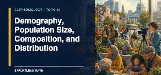
Chapter 14 of the CLEP Sociology study guide on Effortless Math covers Demography, Population Size, Composition, and Distribution: the key terms, the core ideas, and worked examples showing how this topic is tested on the exam.

CLEP Sociology – Chapter 14
Demography, Population Size, Composition, and Distribution
CLEP Introductory Sociology · Chapter 14
Demography, Population Size, Composition, and Distribution
Demography is the systematic study of human populations. Demographers examine population size, composition, and distribution, then study how fertility, mortality, and migration change those features over time.
Population size is the number of people within a defined boundary at a stated time. The boundary can be a neighborhood, city, metropolitan region, country, or another territory. A city can lose residents while its metropolitan region grows because the same move crosses one boundary but stays inside the other.
Population composition describes characteristics such as age, sex, household form, race or ethnicity, education, occupation, or nativity. Composition matters because two places with the same population total can have different needs. A younger population may need more schools, while an older population may need accessible housing and chronic-care services.
Population distribution describes where people live across space. National growth can coexist with regional decline when new jobs and migrants concentrate in a few areas. Infrastructure is local, so a stable national total can hide crowded suburbs, shrinking towns, and neighborhoods with empty housing.
Three processes change population. Fertility concerns actual childbearing in a population. Mortality concerns deaths. Migration changes usual residence. Births and in-migration add residents, while deaths and out-migration remove them from the defined place.
The population balancing equation is
population change=(births-deaths)+(in-migration-out-migration).
The difference between births and deaths is natural increase. It becomes natural decrease when deaths exceed births. Net migration is in-migration minus out-migration. A population can have natural decrease and still grow if positive net migration is larger.
Suppose a region records 12,000 births, 15,000 deaths, 9,000 people moving in, and 4,000 moving out. Natural increase is 12,000-15,000=-3,000. Net migration is 9,000-4,000=5,000. Total population change is -3,000+5,000=2,000, so the region grows by 2,000 even though deaths exceed births.
The same arithmetic change can carry different composition. Two thousand births and two thousand working-age in-migrants both add 2,000 people, yet their immediate effects on schools, employment, housing, and age structure differ. A zero total can hide large movement when gains and losses offset one another.
The time interval must match. Annual births cannot be combined with migration measured over five years. Boundaries must also match. A move from the central city to a suburb counts as out-migration for the city, in-migration for the suburb, and no migration for the wider metropolitan area.
Demography first describes a pattern, then tests explanations. The equation shows how each component contributed. It does not tell why fertility changed, why mortality improved, or why people moved. Those causal questions require evidence about households, institutions, policy, economy, and environment.
Stocks and flows answer different questions. Population size is a stock measured at a point in time. Births, deaths, in-migration, and out-migration are flows recorded during a period. A city can have a large population stock while losing residents during one year, or a small stock while growing quickly. Mixing a one-day population count with a five-year migration total creates a meaningless comparison. Dates and boundaries belong beside every number.
Composition can change even when total size does not. Suppose 5,000 young adults leave a county while 5,000 retirees enter. Net migration is zero, yet age composition, school enrollment, health needs, housing demand, and labor supply may shift. Distribution adds location. If the newcomers settle near a hospital and those leaving came from distant towns, the county’s population geography also changes. On a CLEP item, “how many” asks about size, “who” asks about composition, and “where” asks about distribution. Causes require the next layer of evidence.
Density adds another denominator. Ten thousand residents spread across 100 square miles produce 100 people per square mile, while the same population inside ten square miles produces 1,000. Equal size can therefore accompany very different transport, housing, and service conditions. Keep size, composition, distribution, and density in separate columns when reading a map.
Quick review: Demography studies population size, composition, and distribution. Fertility, mortality, and migration change them. Natural increase is births minus deaths. Net migration is in-migration minus out-migration. Use one boundary and time period before adding the components.
Watch the lesson connection
How Populations Grow and Change gives you a second explanation of the ideas surrounding this lesson. As you watch, pause when the lesson concept appears and explain how the example fits.
Use this lesson for CLEP practice
Write one original example, one close nonexample, and one observation that would help you choose between them. This turns vocabulary recognition into the kind of applied reasoning the exam expects.

Related to This Article
More math articles
- Free Grade 3 English Worksheets for Hawai’i Students
- Geometry Puzzle – Challenge 74
- Organelles and Endosymbiosis
- The Ultimate 6th Grade MAP Math Course (+FREE Worksheets)
- How to Develop Foundational Math Skills for Career Success
- What does SAT Stand for?
- 6th Grade NSCAS Math Worksheets: FREE & Printable
- Top 10 Tips to Overcome PSAT Math Anxiety
- How to Solve Non-Right Triangles Problems
- 6th Grade Ohio’s State Tests Math Worksheets: FREE & Printable














What people say about "Demography, Population Size, Composition | CLEP Sociology"?
No one replied yet.